Easily Create a Drop-Down List in Microsoft Excel: Setup & Customization

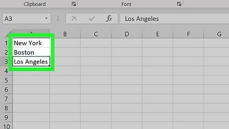
• Create a list of drop-down items in a column. Make sure the items are consecutive (no blank rows).
• Click the cell where you want the drop-down.
• Click the Data Validation button in the Data tab.
• Select the list of drop-down items. Then, customize the list using the data validation options.

Creating a Drop-Down

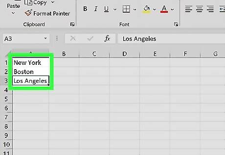
Enter the list of drop-down values in a column. Make sure to enter each drop-down item in a separate, consecutive cell in the same column. For example, if you want your drop-down list to include "New York," "Boston," and "Los Angeles," you can type "New York" in cell A1, "Boston" in cell A2, and "Los Angeles" in cell A3. You can place these items in an existing worksheet, or a new one. They can then be referenced in any worksheet in the workbook. For formatting tips, check out our guide on formatting an Excel spreadsheet.

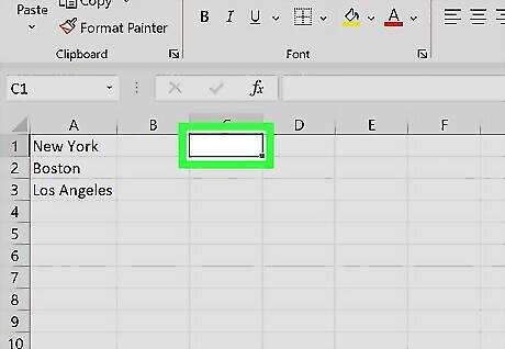
Click the cell where you want to insert your drop-down. This will select the cell. You can insert a drop-down list in any empty cell on your spreadsheet. Drop-downs are helpful for information you want to enter consistently and repeatedly. For example, if you’re making a bill tracker, you could have a drop-down with bill types.

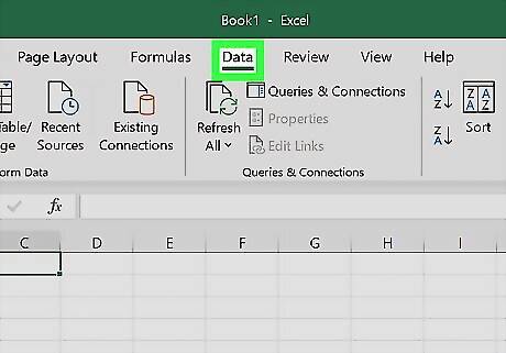
Click the Data tab. You can find this at the top of your spreadsheet. It will open your data tools.

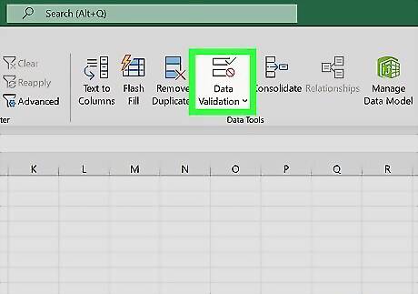
Click the Data Validation. It’s the button on the "Data" toolbar that looks like two separate cells with a green checkmark and a red stop sign.

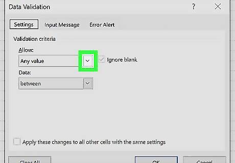
Click the Allow: drop-down. This is in the Settings tab of the Data Validation window.

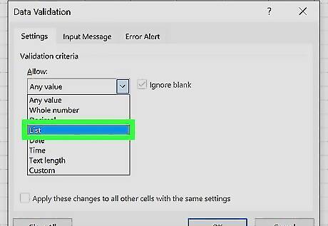
Select List. This option will allow you to create a list in the selected cell.

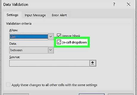
Check the Windows Unchecked In-cell dropdown option. When this option is checked, you will create a drop-down list in the selected cell on your spreadsheet.

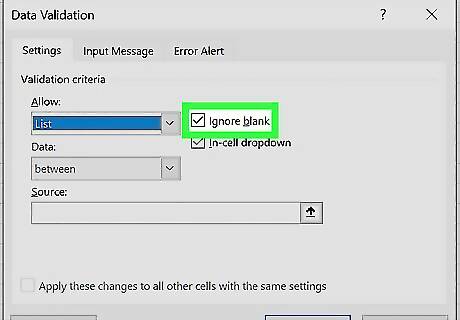
Check the Windows Unchecked Ignore blank option (optional). When this option is checked, users will be able to leave the drop-down empty without an error message. If the drop-down you're creating is a mandatory field, make sure not to check this box.

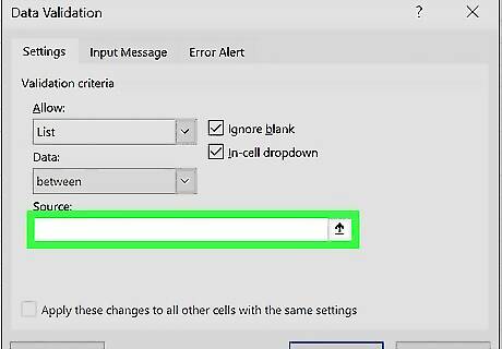
Click the text box under "Source" in the pop-up. You can select the list of values you want in your drop-down. Click the upward arrow button to minimize the Data Validation window, showing only the cell range text box.

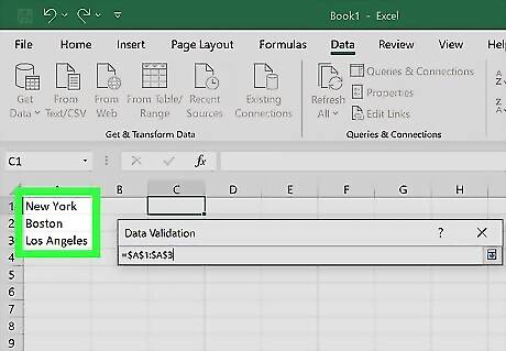
Select your drop-down's list values on the spreadsheet. Click and drag the cursor to select the list of values you want in the drop-down. For example, if you have "New York," "Boston," and "Los Angeles" in cells A1, A2, and A3, make sure to select the cell range from A1 to A3. Alternatively, you can manually type your drop-down list values into the "Source" box here. In this case, make sure to separate each entry with a comma.

Adding List Properties

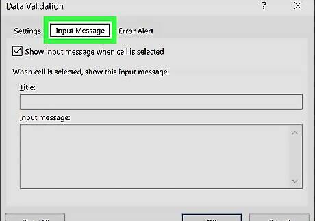
Click Input Message. It's the second tab at the top of the Data Validation window. This tab will allow you to create a pop-up message to display next to your drop-down list.

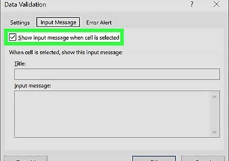
Check Windows Unchecked Show input message when cell is selected. This displays a pop-up message when the drop-down cell is selected. If you don't want to show a pop-up message, just leave the box unchecked.

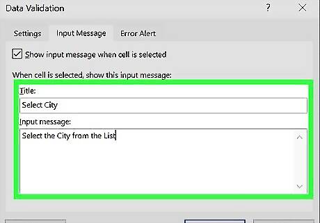
Enter a Title and Input Message. You can use this area to explain, describe or provide more information about the drop-down list. The title and input message you enter here will show up on a small, yellow pop-up sticky note next to the drop-down when the cell is selected.

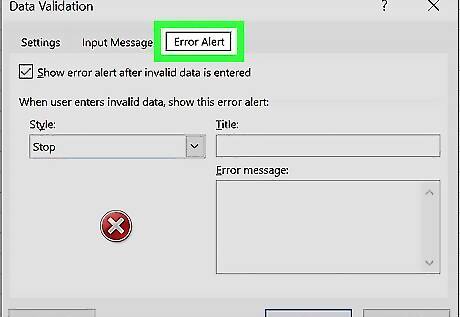
Click Error Alert. This tab will let you display a pop-up error message whenever invalid data is entered into your drop-down cell.

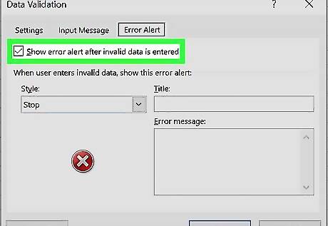
Check Windows Unchecked Show error alert after invalid data is entered. When this option is checked, an error message will pop up when a user types invalid data into the drop-down cell. If you don't want an error message to pop-up, leave the box unchecked.

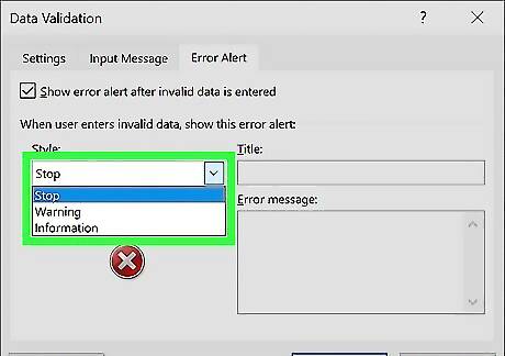
Select an error icon in the Style drop-down. You can select Stop, Warning, or Information. The Stop option will show a pop-up error window with your error message, and stop users from entering data that isn't in the drop-down list. The Warning and Information options will not stop users from entering invalid data, but show an error message with the yellow "!" or blue "i" icon.

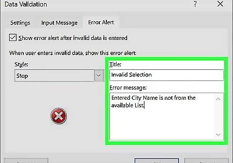
Enter a custom Title and Error message (optional). Your custom error title and message will pop up when invalid data is entered into the drop-down cell. You can leave these fields empty. In this case, the error title and message will default to Microsoft Excel's generic error template. The default error template is titled "Microsoft Excel," and the message reads "The value you entered is not valid. A user has restricted values that can be entered into this cell."

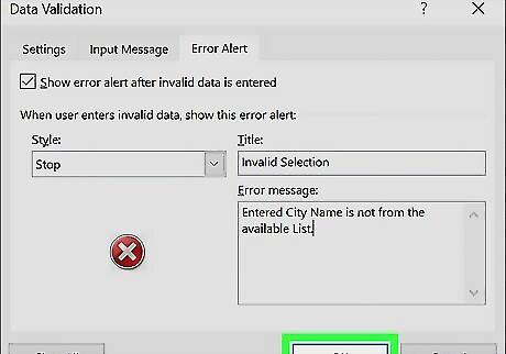
Click OK. This will create and insert your drop-down list into the selected cell. Now users can click the drop-down button (downward triangle) next to the cell to select an item. Make changes to the data validation drop-down list by selecting the cell with the drop-down and clicking the data validation button. The data validation window will reopen and you can edit any of the options. You can copy (ctrl/cmd + c) the cell with the drop-down and paste (ctrl/cmd + v) in other cells to duplicate the drop-down.