views
On Windows

Open your Excel workbook. Double-click the Excel workbook document in which your data is stored. If you don't have the data that you want to analyze in a spreadsheet yet, you'll instead open Excel and click Blank workbook to open a new workbook. You can then enter your data and create a graph from it.
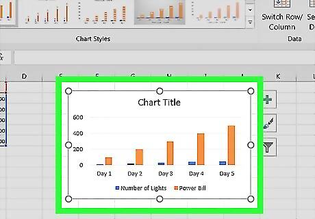
Select your graph. Click the graph to which you want to assign a trendline. If you haven't yet created a graph from your data, create one before continuing.
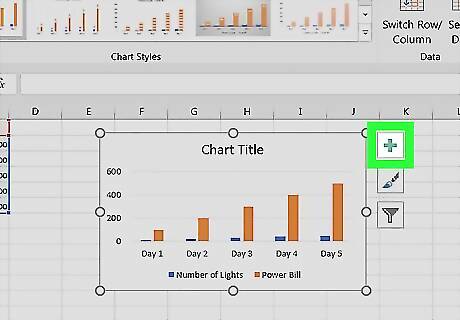
Click +. It's a green button next to the upper-right corner of the graph. A drop-down menu will appear.
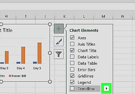
Click the arrow to the right of the "Trendline" box. You may need to hover your mouse over the far-right side of the "Trendline" box to prompt this arrow to appear. Clicking it brings up a second menu.
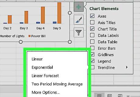
Select a trendline option. Depending on your preferences, click one of the following options Linear Exponential Linear Forecast Two Period Moving Average You can also click More Options... to bring up an advanced options panel after selecting data to analyze.
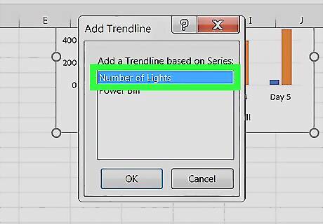
Select data to analyze. Click a data series name (e.g., Series 1) in the pop-up window. If you named your data already, you'll click the data's name instead.
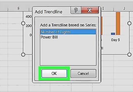
Click OK. It's at the bottom of the pop-up window. Doing so adds a trendline to your graph. If you clicked More Options... earlier, you'll have the option of naming your trendline or changing the trendline's persuasion on the right side of the window.
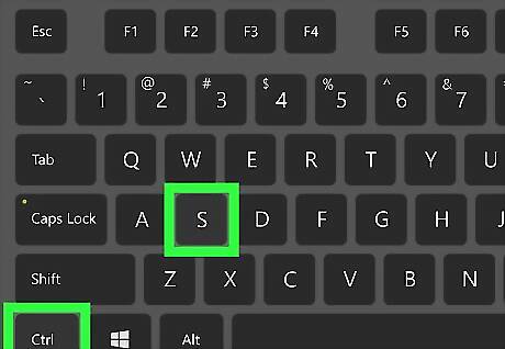
Save your work. Press Ctrl+S to save your changes. If you've never saved this document before, you'll be prompted to select a save location and file name.
On Mac
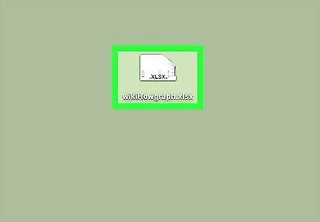
Open your Excel workbook. Double-click the Excel workbook document in which your data is stored. If you don't have the data that you want to analyze in your spreadsheet, you'll instead open Excel to create a new workbook. You can then enter your data and create a graph from it.
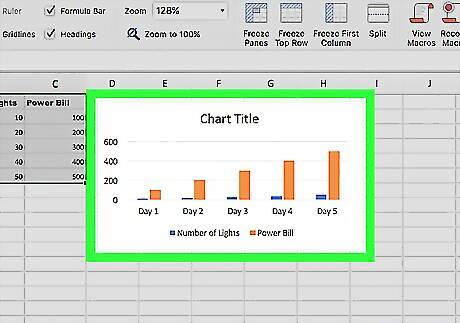
Select the data in your graph. Click the series of data that you want to analyze to select it. If you haven't yet created a graph from your data, create one before continuing.
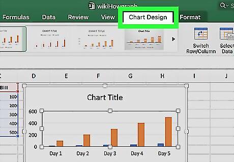
Click the Chart Design tab. It's at the top of the Excel window.
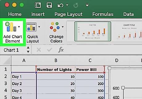
Click Add Chart Element. This option is on the far-left side of the Chart Design toolbar. Clicking it prompts a drop-down menu.
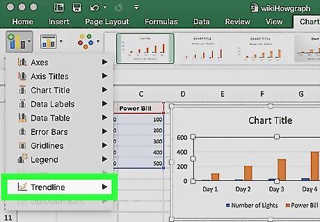
Select Trendline. It's at the bottom of the drop-down menu. A pop-out menu will appear.
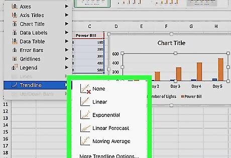
Select a trendline option. Depending on your preferences, click one of the following options in the pop-out menu: Linear Exponential Linear Forecast Moving Average You can also click More Trendline Options to bring up a window with advanced options (e.g., trendline name).
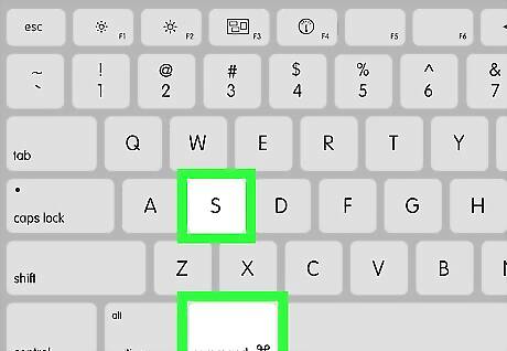
Save your changes. Press ⌘ Command+Save, or click File and then click Save. If you've never saved this document before, you'll be prompted to select a save location and file name.


Comments
0 comment