How to Freeze (Lock in Place) a Cell in Excel

NewsMatrix

Editor

posted on 10 years ago — updated on 1 second ago

35
views

Freezing rows and columns in Microsoft Excel versions 2013, 2010, and 2007 can be helpful if you want to keep a section of your spreadsheet visible at all times while you move to and work in other sections of your document. Individual cells cannot be frozen and locked into place; however, you can freeze one or multiple rows and columns located at the very top and left sides of your spreadsheet, respectively.

Steps

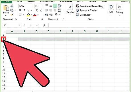
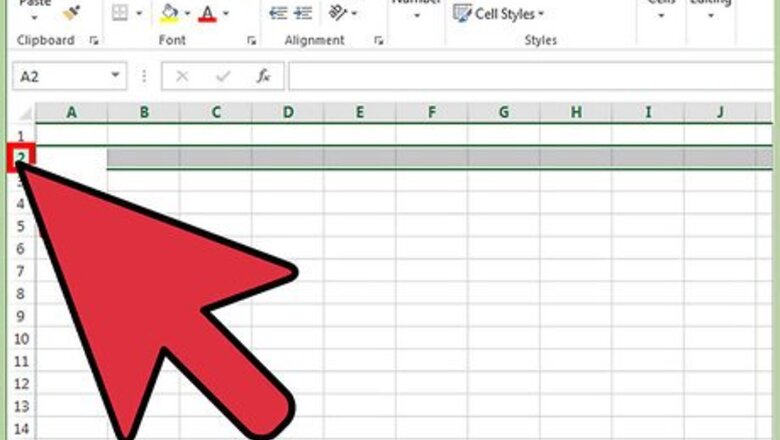
Select the row(s) or column(s) located just below or to the right of the row(s) or column(s) you want frozen. For example, if you want to freeze row 1, select row 2. When freezing a row(s) and column(s) at the same time, click on the one cell located just below and to the right of the row(s) and column(s) you want frozen. For example, if you want to freeze row 1 and column A, click on the cell located in B2.

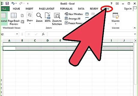
Click on the tab labeled “View” at the top of your Excel session.

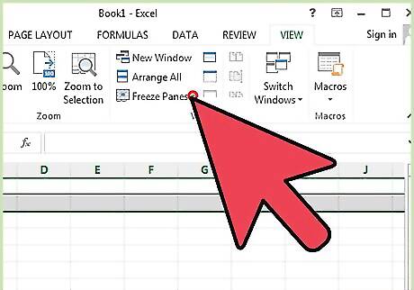
Click on the small arrow next to “Freeze Panes” located in the Window group.

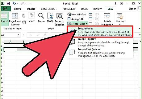
Click on “Freeze Top Row” or “Freeze First Column,” based on your selection. The row(s) and/or column(s) you have selected will now be frozen in place. Select “Freeze Panes” when freezing a row(s) and column(s) at the same time.