How to Calculate Contour Integrals

Direct Parameterization

Apply the Riemann sum definition for contour integrals. Definition. Given a complex function f ( z ) {\displaystyle f(z)} f(z) and a contour γ , {\displaystyle \gamma ,} \gamma , the integral of f ( z ) {\displaystyle f(z)} f(z) over γ {\displaystyle \gamma } \gamma is said to be the Riemann sum lim n → ∞ ∑ i = 0 n f ( z i ) Δ z i . {\displaystyle \lim _{n\to \infty }\sum _{i=0}^{n}f(z_{i})\Delta z_{i}.} \lim _{{n\to \infty }}\sum _{{i=0}}^{{n}}f(z_{{i}})\Delta z_{{i}}. If this limit exists, then we say f ( z ) {\displaystyle f(z)} f(z) is integrable on γ . {\displaystyle \gamma .} \gamma . We communicate this by writing ∫ γ f ( z ) d z . {\displaystyle \int _{\gamma }f(z)\mathrm {d} z.} \int _{{\gamma }}f(z){\mathrm {d}}z. Intuitively, this is a very straightforward generalization of the Riemann sum. We are simply adding up rectangles to find the area of a curve, and send the width of the rectangles to 0 such that they become infinitesimally thin.

Rewrite the contour integral in terms of the parameter t {\displaystyle t} t. If we parameterize the contour γ {\displaystyle \gamma } \gamma as z ( t ) , {\displaystyle z(t),} z(t), then by the chain rule, we can equivalently write the integral below. ∫ γ f ( z ) d z = ∫ Δ t f ( z ( t ) ) d z d t d t {\displaystyle \int _{\gamma }f(z)\mathrm {d} z=\int _{\Delta t}f(z(t)){\frac {\mathrm {d} z}{\mathrm {d} t}}\mathrm {d} t} \int _{{\gamma }}f(z){\mathrm {d}}z=\int _{{\Delta t}}f(z(t)){\frac {{\mathrm {d}}z}{{\mathrm {d}}t}}{\mathrm {d}}t This is the integral that we use to compute. An important note is that this integral can be written in terms of its real and imaginary parts, like so. ∫ Δ t f ( z ( t ) ) d z d t d t = ∫ Δ t ( u ( t ) + i v ( t ) ) d t {\displaystyle \int _{\Delta t}f(z(t)){\frac {\mathrm {d} z}{\mathrm {d} t}}\mathrm {d} t=\int _{\Delta t}(u(t)+iv(t))\mathrm {d} t} \int _{{\Delta t}}f(z(t)){\frac {{\mathrm {d}}z}{{\mathrm {d}}t}}{\mathrm {d}}t=\int _{{\Delta t}}(u(t)+iv(t)){\mathrm {d}}t

Parameterize γ {\displaystyle \gamma } \gamma and calculate d z d t {\displaystyle {\frac {\mathrm {d} z}{\mathrm {d} t}}} {\frac {{\mathrm {d}}z}{{\mathrm {d}}t}}. The simplest contours that are used in complex analysis are line and circle contours. It is often desired, for simplicity, to parameterize a line such that 0 ≤ t ≤ 1. {\displaystyle 0\leq t\leq 1.} 0\leq t\leq 1. Given a starting point z 1 {\displaystyle z_{1}} z_{{1}} and an endpoint z 2 , {\displaystyle z_{2},} z_{{2}}, such a contour can generally be parameterized in the following manner. z ( t ) = ( 1 − t ) z 1 + z 2 , 0 ≤ t ≤ 1 {\displaystyle z(t)=(1-t)z_{1}+z_{2},\ \ 0\leq t\leq 1} z(t)=(1-t)z_{{1}}+z_{{2}},\ \ 0\leq t\leq 1 A circle contour can be parameterized in a straightforward manner as well, as long as we keep track of the orientation of the contour. Let z 0 {\displaystyle z_{0}} z_{{0}} be the center of the circle and r {\displaystyle r} r be the radius of the circle. Then the parameterization of the circle, starting from t = 0 , {\displaystyle t=0,} t=0, and traversing the contour in the counterclockwise direction, is as such. z ( t ) = z 0 + r e i t , 0 ≤ t ≤ 2 π {\displaystyle z(t)=z_{0}+re^{it},\ \ 0\leq t\leq 2\pi } z(t)=z_{{0}}+re^{{it}},\ \ 0\leq t\leq 2\pi Calculating d z d t {\displaystyle {\frac {\mathrm {d} z}{\mathrm {d} t}}} {\frac {{\mathrm {d}}z}{{\mathrm {d}}t}} from both of these contours is trivial. There are two important facts to consider here. First, the contour integral ∫ γ f ( z ) d z {\displaystyle \int _{\gamma }f(z)\mathrm {d} z} \int _{{\gamma }}f(z){\mathrm {d}}z is independent of parameterization so long as the direction of γ {\displaystyle \gamma } \gamma stays the same. This means that there are an infinite number of ways to parameterize a given curve, since the velocity can vary in an arbitrary way. Second, reversing the direction of the contour negates the integral. ∫ − γ f ( z ) d z = − ∫ γ f ( z ) d z {\displaystyle \int _{-\gamma }f(z)\mathrm {d} z=-\int _{\gamma }f(z)\mathrm {d} z} \int _{{-\gamma }}f(z){\mathrm {d}}z=-\int _{{\gamma }}f(z){\mathrm {d}}z

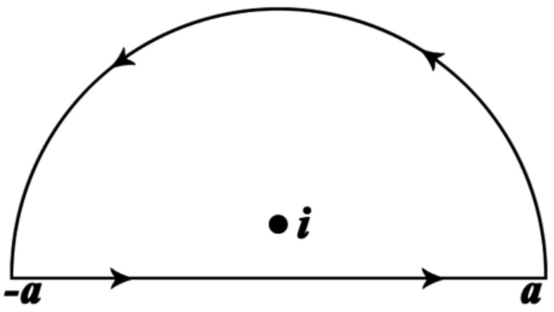
Evaluate. We know that t {\displaystyle t} t is real-valued, so all that remains is to integrate using the standard integration techniques of real-variable calculus. The visual above shows a typical contour on the complex plane. Starting from the point a , {\displaystyle a,} a, the contour traverses a semicircle in the counterclockwise direction with radius a {\displaystyle a} a and closes the loop with a line going from − a {\displaystyle -a} -a to a . {\displaystyle a.} a. If the point z = i {\displaystyle z=i} z=i as shown is taken to be the pole of a function, then the contour integral describes a contour going around the pole. This type of integration is extremely common in complex analysis.

Example

Evaluate the following contour integral. γ {\displaystyle \gamma } \gamma is the curve connecting the origin to 1 + i {\displaystyle 1+i} 1+i along a straight line. ∫ γ ( x y 2 + 2 x y i ) d z {\displaystyle \int _{\gamma }(xy^{2}+2xyi)\mathrm {d} z} \int _{{\gamma }}(xy^{{2}}+2xyi){\mathrm {d}}z

Parameterize the contour. Our curve is especially simple: x = t {\displaystyle x=t} x=t and y = t . {\displaystyle y=t.} y=t. So we write our contour in the following manner. z ( t ) = t + i t , 0 ≤ t ≤ 1 {\displaystyle z(t)=t+it,\ \ 0\leq t\leq 1} z(t)=t+it,\ \ 0\leq t\leq 1

Calculate d z d t {\displaystyle {\frac {\mathrm {d} z}{\mathrm {d} t}}} {\frac {{\mathrm {d}}z}{{\mathrm {d}}t}}. Substitute our results into the integral. d z d t = 1 + i {\displaystyle {\frac {\mathrm {d} z}{\mathrm {d} t}}=1+i} {\frac {{\mathrm {d}}z}{{\mathrm {d}}t}}=1+i ∫ γ ( x y 2 + 2 x y i ) d z = ∫ 0 1 ( t 3 + i 2 t 2 ) ( 1 + i ) d t {\displaystyle \int _{\gamma }(xy^{2}+2xyi)\mathrm {d} z=\int _{0}^{1}(t^{3}+i2t^{2})(1+i)\mathrm {d} t} \int _{{\gamma }}(xy^{{2}}+2xyi){\mathrm {d}}z=\int _{{0}}^{{1}}(t^{{3}}+i2t^{{2}})(1+i){\mathrm {d}}t

Evaluate. ∫ 0 1 ( t 3 + i 2 t 2 ) ( 1 + i ) d t = ∫ 0 1 ( t 3 + i 2 t 2 + i t 3 − 2 t 2 ) d t = 1 4 + i ( 2 3 + 1 4 ) − 2 3 = − 5 12 + 11 12 i {\displaystyle {\begin{aligned}\int _{0}^{1}(t^{3}+i2t^{2})(1+i)\mathrm {d} t&=\int _{0}^{1}(t^{3}+i2t^{2}+it^{3}-2t^{2})\mathrm {d} t\\&={\frac {1}{4}}+i\left({\frac {2}{3}}+{\frac {1}{4}}\right)-{\frac {2}{3}}\\&=-{\frac {5}{12}}+{\frac {11}{12}}i\end{aligned}}} {\begin{aligned}\int _{{0}}^{{1}}(t^{{3}}+i2t^{{2}})(1+i){\mathrm {d}}t&=\int _{{0}}^{{1}}(t^{{3}}+i2t^{{2}}+it^{{3}}-2t^{{2}}){\mathrm {d}}t\\&={\frac {1}{4}}+i\left({\frac {2}{3}}+{\frac {1}{4}}\right)-{\frac {2}{3}}\\&=-{\frac {5}{12}}+{\frac {11}{12}}i\end{aligned}}

Evaluate the same integral, but where γ {\displaystyle \gamma } \gamma is the curve connecting the origin to 1 + i {\displaystyle 1+i} 1+i along y = x 3 {\displaystyle y=x^{3}} y=x^{{3}}. Our parameterization changes to x = t {\displaystyle x=t} x=t and y = t 3 . {\displaystyle y=t^{3}.} y=t^{{3}}. z ( t ) = t + i t 3 {\displaystyle z(t)=t+it^{3}} z(t)=t+it^{{3}} d z d t = ( 1 + i 3 t 2 ) d t {\displaystyle {\frac {\mathrm {d} z}{\mathrm {d} t}}=(1+i3t^{2})\mathrm {d} t} {\frac {{\mathrm {d}}z}{{\mathrm {d}}t}}=(1+i3t^{{2}}){\mathrm {d}}t ∫ γ ( x y 2 + 2 x y i ) d z = ∫ 0 1 ( t 7 + i 2 t 4 ) ( 1 + i 3 t 2 ) d t = ∫ 0 1 ( t 7 + i 2 t 4 + i 3 t 9 − 6 t 6 ) d t = 1 8 + i ( 2 5 + 3 10 ) − 6 7 = − 41 56 + 7 10 i {\displaystyle {\begin{aligned}\int _{\gamma }(xy^{2}+2xyi)\mathrm {d} z&=\int _{0}^{1}(t^{7}+i2t^{4})(1+i3t^{2})\mathrm {d} t\\&=\int _{0}^{1}(t^{7}+i2t^{4}+i3t^{9}-6t^{6})\mathrm {d} t\\&={\frac {1}{8}}+i\left({\frac {2}{5}}+{\frac {3}{10}}\right)-{\frac {6}{7}}\\&=-{\frac {41}{56}}+{\frac {7}{10}}i\end{aligned}}} {\begin{aligned}\int _{{\gamma }}(xy^{{2}}+2xyi){\mathrm {d}}z&=\int _{{0}}^{{1}}(t^{{7}}+i2t^{{4}})(1+i3t^{{2}}){\mathrm {d}}t\\&=\int _{{0}}^{{1}}(t^{{7}}+i2t^{{4}}+i3t^{{9}}-6t^{{6}}){\mathrm {d}}t\\&={\frac {1}{8}}+i\left({\frac {2}{5}}+{\frac {3}{10}}\right)-{\frac {6}{7}}\\&=-{\frac {41}{56}}+{\frac {7}{10}}i\end{aligned}} We have shown here that for non-analytic functions such as f ( z ) = x y 2 + 2 x y i , {\displaystyle f(z)=xy^{2}+2xyi,} f(z)=xy^{{2}}+2xyi, the contour integral is dependent on the path chosen. We can show that this function is non-analytic by checking if the real and imaginary parts satisfy the Cauchy-Riemann equations. As ∂ u ∂ x = y 2 {\displaystyle {\frac {\partial u}{\partial x}}=y^{2}} {\frac {\partial u}{\partial x}}=y^{{2}} and ∂ v ∂ y = 2 x , {\displaystyle {\frac {\partial v}{\partial y}}=2x,} {\frac {\partial v}{\partial y}}=2x, this is enough to demonstrate non-analyticity.

Fundamental Theorem of Contour Integrals

Generalize the Fundamental Theorem of Calculus. As it pertains to contour integrals, the theorem is used to easily compute the value of contour integrals so long as we can find an antiderivative. The proof of this theorem is similar to all other fundamental theorem of calculus proofs, but we will not state it here for brevity. Suppose the function f ( z ) {\displaystyle f(z)} f(z) has an antiderivative F ( z ) {\displaystyle F(z)} F(z) such that d d z F ( z ) = f ( z ) {\displaystyle {\frac {\mathrm {d} }{\mathrm {d} z}}F(z)=f(z)} {\frac {{\mathrm {d}}}{{\mathrm {d}}z}}F(z)=f(z) through a domain D , {\displaystyle D,} D, and let γ {\displaystyle \gamma } \gamma be a contour in D , {\displaystyle D,} D, where z 0 {\displaystyle z_{0}} z_{{0}} and z 1 {\displaystyle z_{1}} z_{{1}} are the start and end points of γ , {\displaystyle \gamma ,} \gamma , respectively. Then ∫ γ f ( z ) d z {\displaystyle \int _{\gamma }f(z)\mathrm {d} z} \int _{{\gamma }}f(z){\mathrm {d}}z is independent of path for all continuous paths γ {\displaystyle \gamma } \gamma of finite length, and its value is given by F ( z 1 ) − F ( z 0 ) . {\displaystyle F(z_{1})-F(z_{0}).} F(z_{{1}})-F(z_{{0}}).

Evaluate the following integral by direct parameterization. γ {\displaystyle \gamma } \gamma is the semicircle going counterclockwise from z = − i {\displaystyle z=-i} z=-i to z = i . {\displaystyle z=i.} z=i. ∫ γ z d z {\displaystyle \int _{\gamma }{\sqrt {z}}\mathrm {d} z} \int _{{\gamma }}{\sqrt {z}}{\mathrm {d}}z

Parameterize γ , {\displaystyle \gamma ,} \gamma , find d z d t , {\displaystyle {\frac {\mathrm {d} z}{\mathrm {d} t}},} {\frac {{\mathrm {d}}z}{{\mathrm {d}}t}}, and evaluate. z ( t ) = e i t , − π 2 ≤ t ≤ π 2 {\displaystyle z(t)=e^{it},-{\frac {\pi }{2}}\leq t\leq {\frac {\pi }{2}}} z(t)=e^{{it}},-{\frac {\pi }{2}}\leq t\leq {\frac {\pi }{2}} d z d t = i e i t {\displaystyle {\frac {\mathrm {d} z}{\mathrm {d} t}}=ie^{it}} {\frac {{\mathrm {d}}z}{{\mathrm {d}}t}}=ie^{{it}} ∫ γ z d z = ∫ − π / 2 π / 2 e 1 2 Log ⁡ e i t i e i t d t = i ∫ − π / 2 π / 2 e 3 2 i t d t = 2 3 e 3 2 i t | − π / 2 π / 2 = 2 3 ( e 3 π 4 i − e − 3 π 4 i ) = 2 3 2 i sin ⁡ 3 π 4 = 2 2 3 i {\displaystyle {\begin{aligned}\int _{\gamma }{\sqrt {z}}\mathrm {d} z&=\int _{-\pi /2}^{\pi /2}e^{{\frac {1}{2}}\operatorname {Log} e^{it}}ie^{it}\mathrm {d} t\\&=i\int _{-\pi /2}^{\pi /2}e^{{\frac {3}{2}}it}\mathrm {d} t\\&={\frac {2}{3}}e^{{\frac {3}{2}}it}{\Bigg |}_{-\pi /2}^{\pi /2}\\&={\frac {2}{3}}\left(e^{{\frac {3\pi }{4}}i}-e^{-{\frac {3\pi }{4}}i}\right)\\&={\frac {2}{3}}2i\sin {\frac {3\pi }{4}}\\&={\frac {2{\sqrt {2}}}{3}}i\end{aligned}}} {\begin{aligned}\int _{{\gamma }}{\sqrt {z}}{\mathrm {d}}z&=\int _{{-\pi /2}}^{{\pi /2}}e^{{{\frac {1}{2}}\operatorname {Log}e^{{it}}}}ie^{{it}}{\mathrm {d}}t\\&=i\int _{{-\pi /2}}^{{\pi /2}}e^{{{\frac {3}{2}}it}}{\mathrm {d}}t\\&={\frac {2}{3}}e^{{{\frac {3}{2}}it}}{\Bigg |}_{{-\pi /2}}^{{\pi /2}}\\&={\frac {2}{3}}\left(e^{{{\frac {3\pi }{4}}i}}-e^{{-{\frac {3\pi }{4}}i}}\right)\\&={\frac {2}{3}}2i\sin {\frac {3\pi }{4}}\\&={\frac {2{\sqrt {2}}}{3}}i\end{aligned}}

Evaluate the same integral using the fundamental theorem of contour integrals. However, in this method, the z {\displaystyle {\sqrt {z}}} {\sqrt {z}} in the integrand presents a problem. Since we know that z = e 1 2 Log ⁡ z , {\displaystyle {\sqrt {z}}=e^{{\frac {1}{2}}\operatorname {Log} z},} {\sqrt {z}}=e^{{{\frac {1}{2}}\operatorname {Log}z}}, the presence of the logarithmic function indicates a branch cut over which we cannot integrate. Fortunately, we can choose our branch cut such that our contour is well-defined in our domain. The principal branch of the logarithm, where the branch cut consists of the non-positive real numbers, works in this case, because our contour goes around that branch cut. As long as we recognize the principal logarithm has an argument defined over ( − π , π ] , {\displaystyle (-\pi ,\pi ],} (-\pi ,\pi ], the rest of the steps are simple computations. ∫ γ z d z = 2 3 z 3 / 2 | − i i = 2 3 ( i 3 2 − ( − i ) 3 2 ) = 2 3 ( e 3 2 Log ⁡ i − e 3 2 Log ⁡ ( − i ) ) {\displaystyle {\begin{aligned}\int _{\gamma }{\sqrt {z}}\mathrm {d} z&={\frac {2}{3}}z^{3/2}{\Bigg |}_{-i}^{i}\\&={\frac {2}{3}}\left(i^{\frac {3}{2}}-(-i)^{\frac {3}{2}}\right)\\&={\frac {2}{3}}\left(e^{{\frac {3}{2}}\operatorname {Log} i}-e^{{\frac {3}{2}}\operatorname {Log} (-i)}\right)\end{aligned}}} {\begin{aligned}\int _{{\gamma }}{\sqrt {z}}{\mathrm {d}}z&={\frac {2}{3}}z^{{3/2}}{\Bigg |}_{{-i}}^{{i}}\\&={\frac {2}{3}}\left(i^{{{\frac {3}{2}}}}-(-i)^{{{\frac {3}{2}}}}\right)\\&={\frac {2}{3}}\left(e^{{{\frac {3}{2}}\operatorname {Log}i}}-e^{{{\frac {3}{2}}\operatorname {Log}(-i)}}\right)\end{aligned}} For the principal branch of the logarithm, we see that Log ⁡ i = i π 2 {\displaystyle \operatorname {Log} i=i{\frac {\pi }{2}}} \operatorname {Log}i=i{\frac {\pi }{2}} and Log ⁡ ( − i ) = − i π 2 . {\displaystyle \operatorname {Log} (-i)=-i{\frac {\pi }{2}}.} \operatorname {Log}(-i)=-i{\frac {\pi }{2}}. ∫ γ z d z = 2 3 ( e 3 2 i π 2 − e − 3 2 i π 2 ) = 2 3 ( e 3 π 4 i − e − 3 π 4 i ) = 2 3 2 i sin ⁡ 3 π 4 = 2 2 3 i {\displaystyle {\begin{aligned}\int _{\gamma }{\sqrt {z}}\mathrm {d} z&={\frac {2}{3}}\left(e^{{\frac {3}{2}}i{\frac {\pi }{2}}}-e^{-{\frac {3}{2}}i{\frac {\pi }{2}}}\right)\\&={\frac {2}{3}}\left(e^{{\frac {3\pi }{4}}i}-e^{-{\frac {3\pi }{4}}i}\right)\\&={\frac {2}{3}}2i\sin {\frac {3\pi }{4}}\\&={\frac {2{\sqrt {2}}}{3}}i\end{aligned}}} {\begin{aligned}\int _{{\gamma }}{\sqrt {z}}{\mathrm {d}}z&={\frac {2}{3}}\left(e^{{{\frac {3}{2}}i{\frac {\pi }{2}}}}-e^{{-{\frac {3}{2}}i{\frac {\pi }{2}}}}\right)\\&={\frac {2}{3}}\left(e^{{{\frac {3\pi }{4}}i}}-e^{{-{\frac {3\pi }{4}}i}}\right)\\&={\frac {2}{3}}2i\sin {\frac {3\pi }{4}}\\&={\frac {2{\sqrt {2}}}{3}}i\end{aligned}}

Original news source