How to Change an Excel Pivot Table Source

SparCzar

Editor

posted on 14 years ago — updated on 1 second ago

9
views

Microsoft's Excel spreadsheet application is designed to allow users to organize and interpret their data using advanced features such as pivot tables, formulas and macros. Occasionally, users of these spreadsheets may need to edit or alter the data in order to answer questions about the results. Changing the source of a pivot table can be confusing, because the source material is typically on a separate sheet, but it is possible to change the source data without losing the formatting of your table.

Steps

Launch Microsoft Excel. You can use either the desktop icon, the Programs listed in the Start menu or the Quick Launch taskbar, depending on your desktop arrangement.

Open the file containing the pivot table and data.

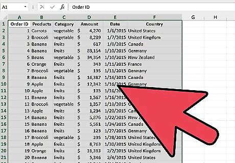
Make any necessary adjustments to the source data. You may need to insert or delete columns and rows. Ensure that all inserted columns have a descriptive heading.

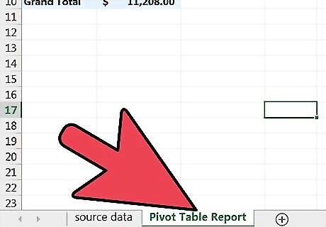
Select the workbook sheet that contains the pivot table by clicking the appropriate tab.

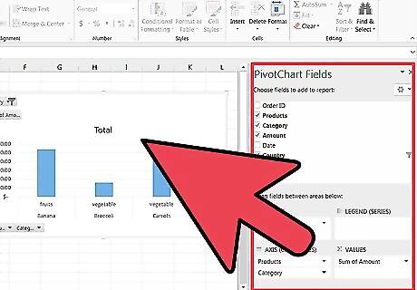
Click inside the pivot table to force the pivot table tools menu to launch. In Excel 2007 and 2010, you will see the Pivot Table Tools menu appear, highlighted in red, above the Options and Design tabs in the ribbon. In Excel 2003, choose "Pivot Table and Pivot Chart Reports" from the Data menu.

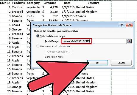
Edit the source data range for your pivot table. In Excel 2007 and 2010, choose "Change Data Source" from the Data group of options. In Excel 2003, launch the Wizard utility by right-clicking inside the pivot table and choosing "Wizard" from the pop-up menu. Click the "Next" button until you see the screen with the source data range. In all versions of Excel, with the source data range highlighted, click and drag to highlight the new range for your data. You can also the range description to include more columns and rows.

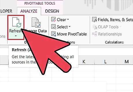
Refresh the pivot table by clicking the "Refresh" button. This button may have a red exclamation point icon, a green "recycle" icon or simply the word "Refresh," depending upon your version and degree of personalization of Excel.