

Using the Alternating Colors Menu

Open Google Sheets. It's the green icon with a white outline of a spreadsheet inside. You'll usually find it in the app drawer.

Tap the spreadsheet you want to edit. Its contents will appear.
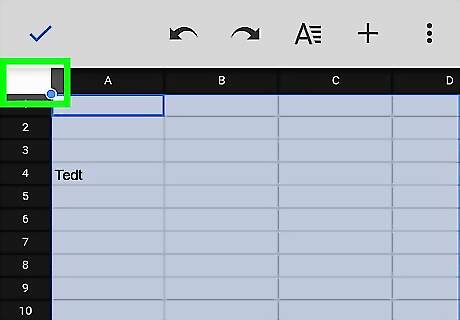
Tap the gray box at the top-left corner of the spreadsheet. It's above the first row and to the left of the first column. This highlights the entire spreadsheet.
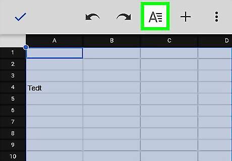
Tap the formatting icon. It's the “A” with several lines at the top the screen. This opens the formatting menu at the bottom of the screen.
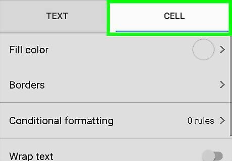
Tap the CELL tab. It's at the top-right corner of the formatting menu.
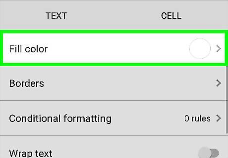
Tap Alternating colors.

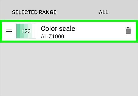
Type the range into the “Apply to range” field. If you want to apply alternating colored rows to the entire sheet you can skip this step, as the range is already filled in.
Tap whether your spreadsheet has a header or footer. For example, if you have a row at the top of the spreadsheet that contains column headings and should not be colored differently, make sure “Header” is switched to On.
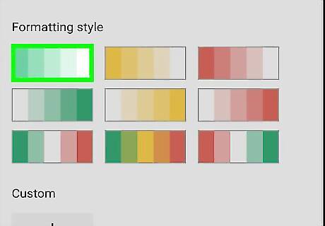
Tap a color scheme. A preview will appear at the top of the screen.

Tap Android 7 Done. It's at the top-left corner of the menu. This saves your selection.
Tap Android 7 Done. It's at the top-left corner of the screen. Every other row of the sheet is now an alternating color.
Using Conditional Formatting

Open Google Sheets. It's the green icon with a white outline of a spreadsheet inside. You'll usually find it in the app drawer.
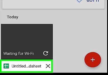
Tap the spreadsheet you want to edit. Its contents will appear.

Tap the gray box at the top-left corner of the spreadsheet. It's above the first row and to the left of the first column. This highlights the entire spreadsheet.

Tap the formatting icon. It's the “A” with several lines at the top the screen. This opens the formatting menu at the bottom of the screen.
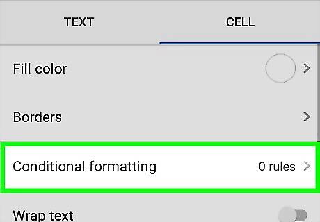
Scroll down the menu and tap Conditional formatting. This opens the “Create a rule” screen.
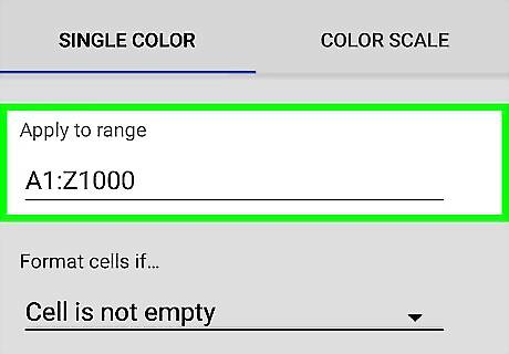
Type the range into the “Apply to range” field. If you want to apply alternating colored rows to the entire sheet you can skip this step, as the range is already filled in.
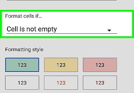
Tap the “Format cells if…” drop-down menu.
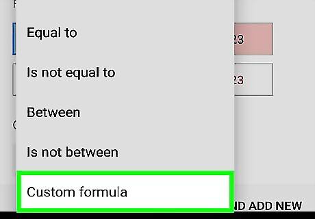
Select Custom formula. It's the final option in the menu.
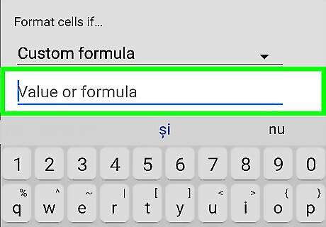
Type =ISEVEN(ROW()) into the blank.
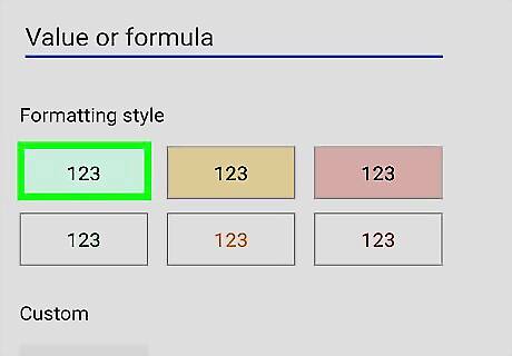
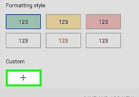
Tap your preferred color for the alternating colored row. The top row of options will color the background of each cell, while the bottom row colors the text.
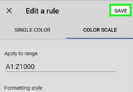
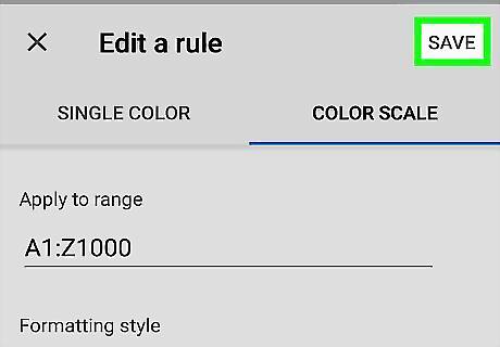
Tap SAVE. It's at the top-right corner of the screen.
Tap Android 7 Done. It's at the top-left corner of the screen. Every other row of the sheet is now an alternating color.


Comments
0 comment