views
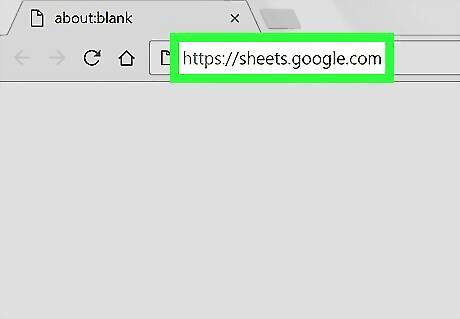
Open Google Sheets in your internet browser. Type sheets.google.com into the address bar, and hit ↵ Enter or ⏎ Return on your keyboard.
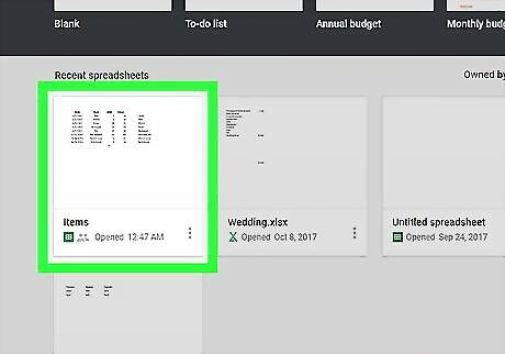
Click the file you want to edit. Find the file you want to highlight in the list of your saved spreadsheet files, and open it.
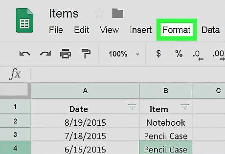
Click the Format tab. This button is on a tabs bar below the file name in the upper-left corner of your spreadsheet. It will open a drop-down menu.
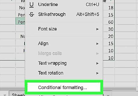
Click Conditional formatting on the Format menu. This will open the formatting panel on the right-hand side of your spreadsheet.
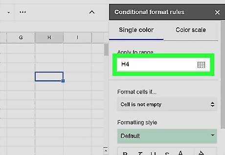
Click the text field under the "Apply to range" heading. This field is at the top of the formatting panel on the right-hand side. It will allow you to select the area you want to edit and highlight.
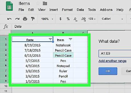
Select the area you want to edit on the spreadsheet. Click your first cell, and drag your mouse to select the area you want to edit. When you click a cell, a new window titled "What data?" will pop-up. You can see your selected cell range in this pop-up window.
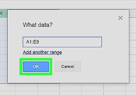
Click OK in the pop-up. This will confirm your range selection.
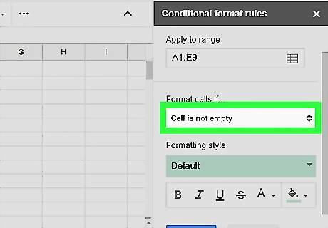
Click the drop-down menu under the "Format cells if" heading. This option is in the middle of the formatting panel on the right-hand side. It will open a list of available formatting conditions.
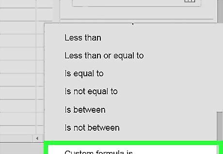
Scroll down and select Custom formula is on the menu. This will allow you to type in a custom formatting formula.
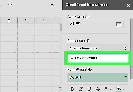
Click the Value or formula field in the formatting panel. You can type in your custom formula here.
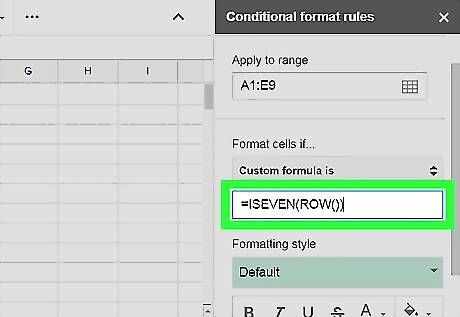
Enter =ISEVEN(ROW()) into the Value or formula field. This formula will highlight all the even-numbered rows in the selected cell range. If the formula above highlights the wrong set of rows, try =ISODD(ROW()). This will highlight all the odd-numbered rows in the selected range. You can find all the row numbers on the left-hand side of your spreadsheet.
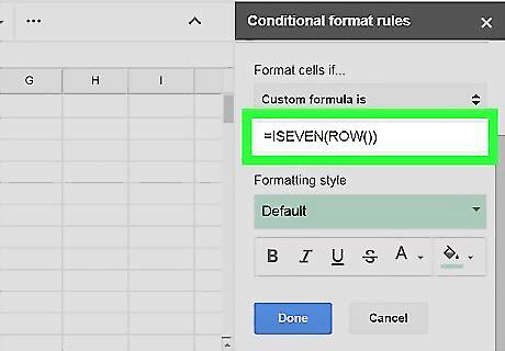
Click the color menu under the "Formatting style" heading. The drop-down menu is green by default. This will open a pop-up window, and allow you to choose a different highlight color.
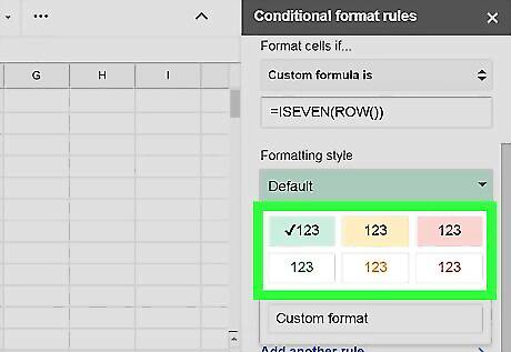
Select a highlight color in the pop-up window. Clicking a highlight color here will automatically apply it to your spreadsheet.
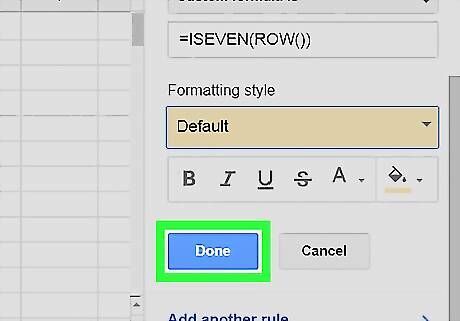
Click the blue Done button. This button is at the bottom of the formatting panel. It will save your new formatting formula. This button doesn't save your changes to the spreadsheet file. Make sure you save all the changes before quitting.


Comments
0 comment